Training ChessMarro
Chess is a great example for learning AI model creation because it has well-defined rules, a finite and discrete state space, and a deterministic nature, making it easier to model computationally. It has been a historical benchmark for AI, from Deep Blue to AlphaZero, offering rich literature and frameworks. The game’s complexity scales from simple moves to deep strategic planning, providing a natural learning curve. Additionally, vast databases of chess games make training AI models more accessible.
We are developing an AI model to determine the best next move in a given chess position, focusing on deep learning methods that have proven competitive against traditional stochastic algorithms. In concrete we are going to make a generic CNN for chess that:
- Will be able to play with only white moves. Black moves will be predicted by invert the board.
- Will be able to play at any point of the game. But:
- There will be more similar starts (logicaly) and we will have special care in mates, so we will put part of our mates database.
- Will predict a legal move before testing.
- Will improve as we can the CNN and hyperparameters.
To develop a chess-playing AI, we can explore several strategies:
-
Neural Network Learning from Historical Data:
- Utilize a neural network trained on a database of chess moves to predict optimal plays based on a given board position. The network takes the current board state as input and selects a move. This move is then compared with the best move from historical examples, and the accuracy is calculated to adjust the neural network for the next example. To enhance this approach, include legal moves as part of the input and properly encode the output in a format compatible with these legal moves.
-
Competing Against Another Chess AI (e.g., Stockfish):
- Engage the neural network in competition against another AI, such as Stockfish. Each decision made by the neural network is scored based on its success. Subsequently, retrain the network using these scores and pit it against the opponent again. Success can be measured by either winning the game or evaluating its moves using a scoring algorithm like Stockfish's.
-
Self-Competition Learning (Inspired by AlphaZero):
- Allow the neural network to compete against itself, with the better versions consistently outperforming the weaker ones. This approach, akin to AlphaZero, is more complex and resource-intensive but offers adaptability to various games and isn't constrained by the opinions of other AIs.
Our choice is the firts one for two principal reasons:
- Can be used with human samples and used in a VET competition using datasets made by students.
- Is "cheap" in tems of required machine and time to train.
*** Lectures ***
- https://www.freecodecamp.org/news/create-a-self-playing-ai-chess-engine-from-scratch/
- http://cs230.stanford.edu/projects_winter_2019/reports/15808948.pdf
- https://ai.stackexchange.com/questions/27336/how-does-the-alpha-zeros-move-encoding-work
- http://www.diva-portal.se/smash/get/diva2:1366229/FULLTEXT01.pdf
- https://github.com/asdfjkl/neural_network_chess/releases
What is a CNN?
A CNN (Convolutional Neural Network) is a type of computer program that helps machines recognize patterns in pictures and videos. It's like a super-smart eye for computers!
Imagine you are looking at a picture of a dog. Your brain automatically sees the fur, ears, and eyes and knows it's a dog. A CNN does something similar but in a digital way. It scans the picture in small parts, finds important details (like shapes, edges, and colors), and then puts everything together to figure out what’s in the image.
CNNs are used in things like facial recognition (unlocking phones with your face), self-driving cars (detecting people and objects), and even medical scans (helping doctors find diseases). So, they help computers "see" and understand the world just like humans do.
Why we will use CNN for Chess moves prediction?
Using a Convolutional Neural Network (CNN) for chess move prediction makes sense because a chessboard is like an image—a grid-based structure where pieces have specific positions, similar to pixels in an image. Here’s why CNNs work well for this task:
-
Chessboard is a Spatial Grid
- A chessboard is an 8x8 grid, just like an image has pixels arranged in rows and columns.
- CNNs are great at detecting patterns in spatial data, so they can analyze piece positions and relationships effectively.
-
Pattern Recognition in Chess
- Chess strategies involve recognizing common patterns, like forks, pins, checkmate threats, and openings.
- CNNs learn from thousands of games, identifying these patterns and predicting the best moves.
-
Local Feature Extraction
- In an image, CNNs detect features like edges and textures.
- In chess, CNNs detect piece clusters, threats, and control over squares, which helps in move prediction.
-
Efficient Processing
- Instead of treating the board as just numbers, CNNs process it like an image, reducing complexity and making training faster.
- They can focus on important regions (like areas around the king in check situations) rather than considering all moves equally.
-
Used in AI Chess Engines
- AI systems like AlphaZero (by DeepMind) use deep learning (including CNNs) to predict chess moves without human-made rules, learning purely from playing games.
- CNNs help AI evaluate positions and choose the best move just like grandmasters do.
We are going to create a CNN (Convolutional Neural Network) to help predict chess moves, similar to how AlphaZero and Leela Chess Zero work.
The main difference is that these powerful AIs learn by playing against themselves over and over, improving with each game. However, in our case, we will train our CNN using games played by you as examples. This will help the AI learn from real human moves.
We need to figure out how to represent the chessboard and the best predicted move so the AI can understand them. Then, we’ll need to create a dataset with different chess positions to train our CNN.
On top of that, we must make sure the moves the AI suggests are valid, meaning they follow the rules of chess, and also check if they are actually good moves.
Preparing the data
We can represent a chess game in varios formats: FEN, FEN moves, SAN moves, UCI moves... and with matrix. Each piece has a letter and we can make a matrix like this:
       +------------------------+
     8 | r  n  b  q  k  b  n  r |
     7 | p  p  p  p  .  p  p  p |
     6 | .  .  .  .  .  .  .  . |
     5 | .  .  .  .  p  .  .  . |
     4 | .  .  .  .  P  P  .  . |
     3 | .  .  .  .  .  .  .  . |
     2 | P  P  P  P  .  .  P  P |
     1 | R  N  B  Q  K  B  N  R |
       +------------------------+
         a  b  c  d  e  f  g  h'
To train a Convolutional Neural Network (CNN) to predict chess moves, we need to represent the chessboard in a way the AI can understand.
At first, we might think of using a single matrix (grid of numbers) like this:
[
  [ 4,  2,  3,  5,  6,  3,  2,  4],
  [ 1,  1,  1,  1,  0,  1,  1,  1],
  [ 0,  0,  0,  0,  0,  0,  0,  0],
  [ 0,  0,  0,  0, -1,  0,  0,  0],
  [ 0,  0,  0,  0, -1, -1,  0,  0],
  [ 0,  0,  0,  0,  0,  0,  0,  0],
  [-1, -1, -1, -1,  0, -1, -1, -1],
  [-4, -2, -3, -5, -6, -3, -2, -4]
]
Here:
- Positive numbers represent white pieces.
- Negative numbers represent black pieces.
- Different numbers represent different pieces (pawns, knights, bishops, etc.).
Why is This a Problem?
The CNN might misinterpret the numbers because it learns based on patterns and weights. For example:
- The number 6 (king) is much bigger than 1 (pawn), but in chess, every piece is important!
- A CNN might think higher numbers mean more important pieces, which is not true in all situations.
A Better Solution: One Matrix for Each Piece Type
Instead of using a single matrix, we use separate matrices for each type of piece. For example:
- One matrix for pawns
- One matrix for knights
- One matrix for bishops
- One matrix for rooks
- One matrix for queens
- One matrix for kings
Each matrix is filled with 1s and 0s. This way, all pieces are treated equally, and the CNN can better understand their positions.
- The AI sees chess like an image, where each type of piece has its own layer, just like different colors in a picture.
- It prevents the AI from making mistakes based on number size.
- It improves move predictions by focusing on piece positions, not their values.
       [[[0., 0., 0., 0., 0., 0., 0., 0.],
         [0., 0., 0., 0., 0., 0., 0., 0.],
         [0., 0., 0., 0., 0., 0., 0., 0.],
         [0., 0., 0., 0., 0., 0., 0., 0.],
         [0., 1., 0., 0., 0., 0., 0., 0.],
         [0., 0., 0., 0., 0., 0., 1., 0.],
         [0., 0., 0., 0., 0., 0., 0., 0.],
         [0., 0., 0., 0., 0., 0., 0., 0.]],

        [[0., 0., 0., 0., 0., 0., 0., 0.],
         [0., 0., 0., 0., 0., 0., 1., 0.],
         [1., 0., 0., 0., 0., 0., 0., 0.],
         [0., 1., 0., 0., 1., 0., 0., 1.],
         [0., 0., 0., 0., 0., 0., 0., 0.],
         [0., 0., 0., 0., 0., 0., 0., 0.],
         [0., 0., 0., 0., 0., 0., 0., 0.],
         [0., 0., 0., 0., 0., 0., 0., 0.]],
         ...
This format is inspired in Alphazero way to code data. Alphazero does it more complex, but it has information about previous moves. But in theory, getting the best move is not related to historic data. Leela zero uses similar aproach.
We don't just look at the chessboard; our representation also tracks all possible moves for each piece. It does this using a multi-channel matrix, meaning there are many separate layers of information about potential moves. Representing all possible legal moves for every piece in a game position. This means the AI will not only know where pieces are but also where they can go, making it smarter in predicting the best move.
Format of the data
When training a chess AI, we need to store a lot of chess games in a way that the computer can understand. However, if we don’t use a smart format, the data can become too large and slow down the training process.
-
Each chess situation is stored in a 77x8x8 matrix
- This means there are 77 layers of 8x8 grids, each storing different details about the board.
- Instead of saving regular numbers, we use a compressed format where each number is a 64-bit integer (int64).
-
Why Use int64 Instead of a Regular 8x8 Grid?
- A normal 8x8 matrix in CSV or JSON takes at least 8 bits per number, plus extra characters like commas, brackets, etc.
- Using int64 (64-bit integer) allows us to store an entire 8x8 matrix using just 1 bit per number—saving a lot of space!
- If the dataset has 100,000 complete chess games, and each game has many moves (each move is a new board position).
- In FEN format (a way to describe chess positions), the dataset is about 500MB.
- In the 77x int64 format, it could be 1.5GB.
- If we stored it in a regular 77x8x8 format, it could be more than 10GB, which is too large!
How Do We Prepare the Data for AI Training? Before training, we need to convert this data into a format the AI can use: ✅ Convert the 77x int64 data into a 76x8x8 NumPy matrix (NumPy is a fast way to handle numbers in Python). ✅ Reduce the dataset size so we can train with more chess games without using too much storage.
This 77 array of matrix represents 77 boards with different type of information each one:
- The 12 first represents the position of the 6 types of pieces x2 colors:
    [
     white pawns, black pawns, white knights, black knights, white bishops, black bishops, white rooks, black rooks, white queen, black queen, white king, black king
    ]
One 1 in a place means this type of piece is on it.
- Then, we have a entire binary matrix that informs about turn. It means a 8x8 1s matrix is Black turn and 8x8 0s matrix is white turn
- The other 64 matrix are for all the possible moves of a piece. Since a queen can do every move except the knights moves, we take as a reference the queen. A queen can potentialy move in 8 directions and can move until 7 positions. This possible moves are the first 56 matrix. The other 8 are the 8 possible moves of a knights
    [
    ...North moves x 7, ...NE x 7, ...E x7, ...SE x7, ...S x7, ...SW x7, ...W x7, ...NW x7  (Queen moves)
    ...knights x 8
    ]
- The other 64 matrix are for all the possible moves of a piece.
In a chess game, different pieces have different movement patterns. For example, a Queen can move in multiple directions, while a Knight has a very unique movement style. We can use a matrix to represent all these possible moves efficiently.
The Queen is one of the most powerful pieces in chess. It can move:
- Vertically (up and down the board)
- Horizontally (left and right)
- Diagonally in all four directions (NE, SE, SW, NW)
The Queen can potentially move up to 7 squares in any of these 8 directions (since the board is 8x8). So, in total, there are 56 possible moves for the Queen:
- 7 moves to the North (Up)
- 7 moves to the North-East (NE)
- 7 moves to the East (Right)
- 7 moves to the South-East (SE)
- 7 moves to the South (Down)
- 7 moves to the South-West (SW)
- 7 moves to the West (Left)
- 7 moves to the North-West (NW)
Each of these 8 directions is represented as a matrix of size 8x8, and the first 56 matrices (out of 64) will be used to describe all possible Queen's moves in these directions.
The Knight has a very unique movement: it moves in an "L" shape, either:
- Two squares in one direction (up/down/left/right), then one square perpendicular to that direction (left/right/up/down).
- Or, one square in one direction (up/down/left/right), then two squares perpendicular to that direction.
There are exactly 8 possible moves for a knight from any given position. These are:
- Two squares up and one square left.
- Two squares up and one square right.
- Two squares down and one square left.
- Two squares down and one square right.
- One square up and two squares left.
- One square up and two squares right.
- One square down and two squares left.
- One square down and two squares right.
The remaining 8 matrices in the representation are used to describe these 8 possible moves for the Knight.
So, if we organize the data:
- The first 56 matrices represent the Queen's possible moves in the 8 directions (North, NE, East, SE, South, SW, West, NW).
- The last 8 matrices represent the Knight's 8 possible moves.
Each matrix is an 8x8 grid where:
- 1 represents a potential move to that square (a valid move for the piece).
- 0 represents a square where the piece cannot move (based on its movement type).
We can visualize the structure of the full 64 matrices like this:
[
  ... 7 North moves x 8,  # First 7 matrices for Queen's North moves
  ... 7 NE moves x 8,     # Next 7 matrices for Queen's NE moves
  ... 7 East moves x 8,   # Next 7 matrices for Queen's East moves
  ... 7 SE moves x 8,     # Next 7 matrices for Queen's SE moves
  ... 7 South moves x 8,  # Next 7 matrices for Queen's South moves
  ... 7 SW moves x 8,     # Next 7 matrices for Queen's SW moves
  ... 7 West moves x 8,   # Next 7 matrices for Queen's West moves
  ... 7 NW moves x 8,     # Next 7 matrices for Queen's NW moves

  ... 8 Knight's possible moves (8 matrices)
]
This fragment of code shows how is created the codes dictionary where each key is a tuple of the move and "i" represents the index of the matrix of each move inside the 64 layers matrix of all the moves:
codes, i = {}, 0
    # All 56 regular moves
for nSquares in range(1,8):
    for direction in [(0,1), (1,1), (1,0), (1,-1), (0,-1), (-1,-1), (-1,0), (-1,1)]:
            codes[(nSquares*direction[0],nSquares*direction[1])] = i
            i += 1
    # 8 Knight moves
codes[(1,2)], i = i,  i+1
codes[(2,1)], i = i,  i+1
codes[(2,-1)], i = i,  i+1
codes[(1,-2)], i = i,  i+1
codes[(-1,-2)], i = i,  i+1
codes[(-2,-1)], i = i,  i+1
codes[(-2,1)], i = i,  i+1
codes[(-1,2)], i = i,  i+1
Why this structure?
Instead of a single numerical matrix, we represent the board state using a tensor. This is composed of:
- 12 Piece Matrices: One for each piece type (Pawn, Knight, Bishop, Rook, Queen, King) per color (White/Black).
- 1 Turn Matrix: A constant layer indicating whose turn it is.
- 64 Movement Matrices: Encoding all potential legal moves for the current board state.
Representing the board as specialized layers is advantageous for a Convolutional Neural Network (CNN) for several reasons:
- Spatial Hierarchies: Since chess is inherently an grid, CNNs excel at detecting spatial patterns (like pin formations, battery attacks, or king safety) that are preserved by this structure.
- Efficient Feature Extraction: Separate matrices allow the model to learn the unique "identity" and tactical value of each piece independently before combining them into higher-level strategic concepts in deeper layers.
- Data Alignment: Aligning the input directly with the physical layout of the board makes the model's decisions more interpretable and simplifies the ETL (Extract, Transform, Load) process.
Understanding Movement Matrices: The "Heat Map" Analogy
To help the AI "visualize" its options, we treat legal moves as image data. Think of each move matrix as a grid of pixels:
- 1 (On): A legal move is possible from/to that square.
- 0 (Off): No move is possible.
A position becomes "hot" when the AI detects a high density of 1s in these matrices. For example, a Queen in the center generates a "hotter" movement signature than a trapped Knight. This serves as a Boolean Mask, ensuring the model prioritizes legal, high-value moves during the training and inference phases.
Our architecture, ChessMarro, optimizes for resource efficiency by simplifying the input space:
- No Historical Data: Unlike AlphaZero, which uses -previous moves, we focus on the current state. This significantly reduces RAM, disk space, and GPU overhead.
- Simplified State: We omit complex tracking (castling rights, repetition) to prioritize a "lighter" model that maintains strong "intuition" (Top-1 accuracy) without the need for massive computational clusters.
Thinking of the Matrix Like a Pixel in an Image
Imagine you have an image on a screen. This image is made up of tiny dots called pixels. Each pixel has a color, and when you combine all these pixels, they form a complete picture. In the same way, we can think of the matrix for chess moves as a grid of tiny "pixels".
In our case, the grid is an 8x8 matrix (like a chessboard). Each square on this chessboard can either be a 1 (a move is possible) or a 0 (no move possible). So, this matrix is like an image where each square can be on (1) or off (0).
Now, think about how we use this grid to represent a piece's movement. Each piece (like a Queen or Knight) has its own pattern of possible moves.
- If a piece can move to a certain square, we mark it with a 1.
- If it can't move there, we mark it with a 0.
For example:
- The Queen can move in many directions (up, down, diagonally), so in the matrix, many squares will have 1s where it can go, and 0s everywhere else.
- The Knight moves in an "L" shape, so only a few squares will have 1s for its possible moves.
The idea of a "hot" position means that the piece is very active or has a lot of potential moves. So, in the matrix:
- The position where the piece is located (like the Queen’s starting position) will have more 1s around it, because the piece can move to more squares.
- The AI will notice that these positions are important because the piece has more options, and that makes the position "hotter".
Best move representation
Lets talk about best move representation:
Best move is represented in a 0 to 4096 format to simplify. And it 's calculated with
    np.ravel_multi_index(
            multi_index=((from_rank, from_file, move_type)),
            dims=(64,8,8)
        )
In chess, each move a piece makes can be represented in a special way. Instead of writing out the move in a regular format (like e2 to e4), we use a system that turns the move into a number between 0 and 4096. This number helps the computer understand all possible moves in a simplified way.
To create this number, we use a function called np.ravel_multi_index, which combines three pieces of information:
from_rank: The row where the piece starts.from_file: The column where the piece starts.move_type: The type of move being made (like a regular move, a capture, or castling).
This function takes these three pieces of information and turns them into a number between 0 and 4095, which corresponds to one of the 4096 possible legal moves in chess. This way, the computer can easily track all possible moves.
We choose this simple way to represent moves to make easy to the CNN to return a prediction because prediction is an array of 4096 numbers that represent the provability of each one to be the best move.
Now, when we give this number to the neural network (AI), it understands it by looking at a matrix (a big grid) of legal moves for every piece on the board. The AI knows that there will always be one active (valid) move to choose, and it can pick the right one based on the piece's position and the available moves.
Additionally, we need to convert between different formats of moves. For example, the moves might be in a UCI format (like e2e4) and we need to turn it into this special number format, or the AI might need to convert the number back into a regular move. This is called coding and decoding the move formats.
This is the function used in our code:
def uci_to_number(uci_move):
    m = uci_move #chess.Move.from_uci(uci_move)
    move_code = codes[(chess.square_file(m.to_square) - chess.square_file(m.from_square),
                   chess.square_rank(m.to_square) - chess.square_rank(m.from_square))]
    pos = np.ravel_multi_index(
        multi_index=((move_code, 7-chess.square_rank(m.from_square), chess.square_file(m.from_square))),
        dims=(64,8,8)
    )
    return pos
And this is the function to convert again to UCI format:
def number_to_uci(number_move):
    move_code, from_row, from_col = np.unravel_index(number_move, (64, 8, 8))  # Rank == row, file== col
    code = list(codes.keys())[list(codes.values()).index(move_code)]
    row_a = str(8-from_row)
    col_a = chr(ord('a') + from_col)
    col_b = chr(ord('a') + from_col + code[0])
    row_b = str(8-from_row + code[1])
    uci_move = f"{col_a}{row_a}{col_b}{row_b}"
    return uci_move
As we can see, it uses codes, the previous dictionary of moves.
Training in a notebook
Here we only are going to see the important code, but in the notebook there are all the code necessary to train and test our model
As all AI projects in Python, we need to import lots of libraries. These are the most common: numpy for numerical jobs, pandas to data management and parquet for data loading and storage. We need to install python-chess and ipython to code chess scenarios and to improve feeback in this notebook.
Reading the data
To read the data we need a function to transform the parquet files in dataframes:
def read_data(file,page,size):
    with pq.ParquetFile(file) as pf:
        print("reading",file, page, size, pf.metadata)

        iterb = pf.iter_batches(batch_size = size)
        for i in range(page):
            next(iterb)

        batches = next(iterb)

        df_chess = pa.Table.from_batches([batches]).to_pandas()

        batches = None
        iterb = None

        # reshape
        df_chess['board'] = df_chess['board'].apply(lambda board: board.reshape(77, 8, 8).astype(int))
        df_chess.info(memory_usage='deep')
        df_chess.memory_usage(deep=True)
        return df_chess
To efficiently manage and feed our extensive collection of chess positions and their corresponding optimal moves into our PyTorch deep learning model, we must define a Custom Dataset class. This class acts as a bridge between our raw data files (like our Parquet dataset of games) and PyTorch’s optimized data pipeline, the DataLoader.
The DataLoader is responsible for high-level tasks such as shuffling the data, batching samples together, and executing parallel data loading (using multiple worker processes). However, it relies entirely on our custom class to understand how to access and process individual data points.
To be compatible with the PyTorch ecosystem, our custom class must inherit from torch.utils.data.Dataset and implement three core methods: init, len, and getitem.
def create_dataLoaders(df_chess):
    # This class is used by pytorch for providing data to model. We use it to read dataset and convert to desired format
    class ChessDataset(Dataset):
        def __init__(self, df):
            self.dataframe = df

        def __len__(self):
            return len(self.dataframe)

        def __getitem__(self, idx):
            fen = torch.tensor(self.dataframe.loc[idx, 'board'], dtype=torch.float32)
            uci_best_move = self.dataframe.loc[idx, 'best']
            return (fen, uci_best_move, self.dataframe.loc[idx, 'fen_original'])


    # We can select a small sample to try the training algorithm
    # In this case we select all the Dataset provided
    df_selected = df_chess.sample(n=len(df_chess), random_state=42).reset_index(drop=True)

    # Then we create an Object with this dataset
    data_train = ChessDataset(df_selected)

    # Select 80% for training and 20% for testing
    train_size = int(0.8 * len(data_train))
    test_size = len(data_train) - train_size
    print(len(data_train))
    train_dataset, test_dataset = torch.utils.data.random_split(data_train, [train_size, test_size])

    # Create the Dataloader
    dataloader = DataLoader(train_dataset, batch_size=32, shuffle=True, drop_last=True)
    dataloader_test = DataLoader(test_dataset, batch_size=32, shuffle=True, drop_last=True)
    return (dataloader, dataloader_test)
Let's break it down so it's easier to understand!
This function prepares the chess game data so that it can be fed into the AI model (a neural network) for training. It does this by creating a custom dataset that works with PyTorch, which is a tool used to build AI models. Here's what each part does:
-
ChessDatasetClass: This class is like a special container that stores the chess game data. It's a format that PyTorch understands.__init__: This is the constructor. It just takes the data from the pandas DataFrame (where we stored the chess data) and saves it inside the class for later use.__len__: This tells PyTorch how many pieces of data are in the dataset. In this case, it returns the number of rows (games) in the DataFrame.__getitem__: This is a very important part. When PyTorch wants to get a specific piece of data, it will call this method. It takes an index number (idx), grabs the data (like the board and the best move) for that index, and returns it in a format that PyTorch can use.
-
Selecting a Sample: To test the AI model quickly, we select a random sample of the data to train on. This is done by using
.sample()to shuffle the data and reset the index so it's in order. -
Splitting into Training and Testing Data: We then split the data into two parts:
- Training data (80%): This is the data the AI will learn from.
- Testing data (20%): This is used to check how well the AI has learned after training.
-
Creating DataLoaders: PyTorch needs to use DataLoaders to efficiently feed the data to the model during training. The DataLoader batches the data into groups (in this case, 32 samples at a time) and shuffles the data to make training more effective. We also make sure that each batch has a fixed size and the data is split properly between training and testing.
-
Return the DataLoaders: Finally, the function returns the training DataLoader and the testing DataLoader, which the model will use to train and test.
In simple terms, this function prepares the chess data, splits it into training and testing sets, and organizes it into a format that the AI model can understand and learn from.
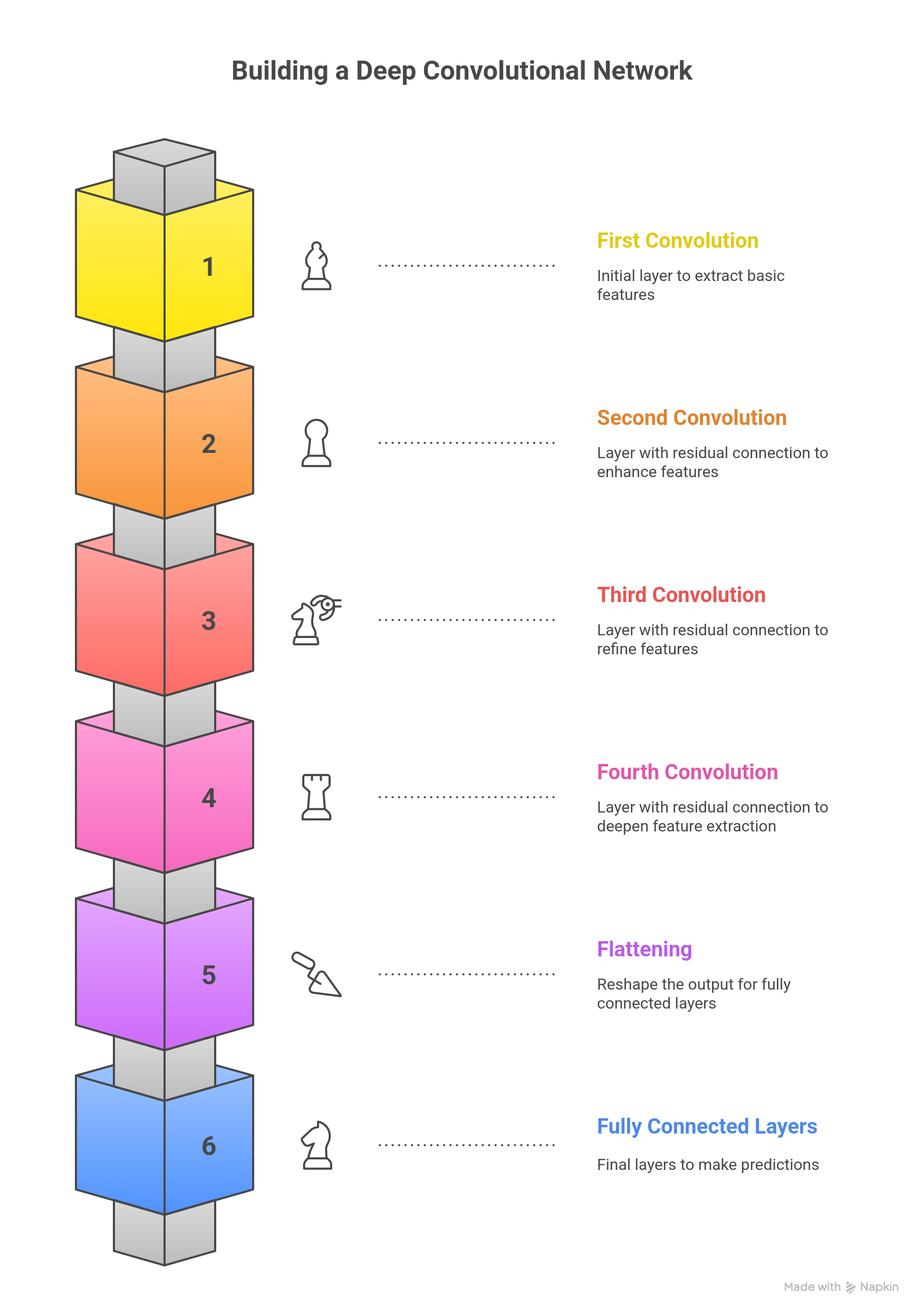
The CNN model Architecture
When building a Convolutional Neural Network (CNN) for chess, we need to define how the AI learns from the data. This part is important because the network’s structure (how many layers, neurons, and connections it has) will determine how well the AI performs.
In this setup, we're basing the model on simpler, well-tested architectures that have been used by other people (like the one in this AlphaZero project). These models have worked well for others, and we're using them as a starting point to save time and resources.
However, there are some key things to consider:
-
Machine Power and Memory: Adding more layers (complexity) to the CNN can make it more powerful, but it also requires more computing resources. It will need more memory and take more time to train. So, it's important to find the right balance between a powerful model and the resources we have available.
-
Performance vs. Efficiency: More layers don't always mean better performance. Sometimes, a simpler model works just as well or even better, depending on the task and data. For example, adding too many layers can make the model slow and might not improve its ability to make good moves. Instead, we focus on keeping the model efficient while still powerful enough to learn from the chess data.
The goal here is to build a network that is strong enough to understand chess, but not so complicated that it becomes slow or too demanding for the computer to handle. The best balance is key to making the AI learn effectively without overloading the system.
Convolutional, Normalization, and Fully Connected layers are the essential building blocks in Deep Learning architectures. Each type of layer plays a critical role in data processing and learning, especially when applied to structured data like a chess board in a Convolutional Neural Network (CNN).
1. Convolutional Layers
- Primary Purpose: To learn spatial and hierarchical patterns from the input data. They are fundamental for processing data with a grid-like topology, such as images or, in our case, the 8x8 chess board representation.
- Key Function: They apply a set of small filters (kernels) to local regions (receptive fields) of the input. This operation generates feature maps that highlight learned patterns (e.g., edges, textures, or specific piece threats in a chess position).
- Key Parameters: Kernel Size, Stride (the step size of the filter), Padding (boundary fill), and the number of Output Channels (i.e., the number of filters).
- Relevance to AI Chess: Crucial for translating the board state into an abstract understanding of strategic patterns (e.g., pawn structures, king safety, or lines of attack/defense).
2. Normalization Layers
- Primary Purpose: To significantly stabilize and accelerate training by mitigating the Internal Covariate Shift phenomenon.
- Key Function: These layers adjust the input to each subsequent layer so that it has a mean close to zero and a standard deviation close to one. This standardization ensures that gradients flow efficiently throughout the deep network.
- Common Types:
- Batch Normalization (BN): Normalizes across the entire mini-batch.
- Layer Normalization (LN): Normalizes across all the activations within a single sample's layer.
- Relevance to AI Chess: Essential for training deeper models like the
ChessNetmentioned in the project files, allowing for higher learning rates and reducing dependency on precise weight initialization.
3. Fully Connected Layers (Dense Layers)
- Primary Purpose: To capture high-level, non-spatial relationships and perform the final linear transformation of the learned features.
- Key Function: Every neuron in this layer is connected to every neuron in the preceding layer. They take the abstract feature maps learned by the convolutions and map them to the final output format required for the problem.
- Key Parameters: Number of Neurons in the layer and the Activation Function (e.g., ReLU, Softmax for classification).
- Relevance to AI Chess: These layers form the "Head" of the AI model, performing the final prediction:
- Policy Head: Uses Softmax to output a probability distribution over the legal next moves.
- Value Head: Uses Tanh or linear activation to output the predicted board evaluation (positional advantage).
This is the code:
class Mish(nn.Module):
    """Activación Mish: x * tanh(softplus(x))"""
    def forward(self, x):
        return x * torch.tanh(F.softplus(x))

class SEBlock(nn.Module):
    """Squeeze-and-Excitation Block para atención de canales"""
    def __init__(self, channels, reduction=16):
        super(SEBlock, self).__init__()
        self.avg_pool = nn.AdaptiveAvgPool2d(1)
        self.fc = nn.Sequential(
            nn.Linear(channels, channels // reduction, bias=False),
            nn.ReLU(inplace=True),
            nn.Linear(channels // reduction, channels, bias=False),
            nn.Sigmoid()
        )

    def forward(self, x):
        b, c, _, _ = x.size()
        y = self.avg_pool(x).view(b, c)
        y = self.fc(y).view(b, c, 1, 1)
        return x * y.expand_as(x)

class ResBlock(nn.Module):
    """Bloque Residual con Pre-activación y SE"""
    def __init__(self, channels):
        super(ResBlock, self).__init__()
        self.bn1 = nn.BatchNorm2d(channels)
        self.conv1 = nn.Conv2d(channels, channels, kernel_size=3, padding=1, bias=False)
        self.bn2 = nn.BatchNorm2d(channels)
        self.conv2 = nn.Conv2d(channels, channels, kernel_size=3, padding=1, bias=False)
        self.se = SEBlock(channels)
        self.activation = Mish()

    def forward(self, x):
        residual = x
        out = self.bn1(x)
        out = self.activation(out)
        out = self.conv1(out)

        out = self.bn2(out)
        out = self.activation(out)
        out = self.conv2(out)

        out = self.se(out)
        return out + residual

class ChessNetPV_Optimized(nn.Module):
    def __init__(self, num_blocks=6): # 6 o 12 bloques es mucho más profundo que el original
        super(ChessNetPV_Optimized, self).__init__()

        in_channels = 77
        base_channels = 256 # Ancho constante profesional
        head_bottleneck_channels = 32 # Para reducir parámetros en FC [6]


        # Entrada inicial
        self.conv_input = nn.Conv2d(in_channels, base_channels, kernel_size=3, padding=1, bias=False)

        # Torre Residual (Cuerpo de la red)
        self.res_tower = nn.Sequential(
            *[ResBlock(base_channels) for _ in range(num_blocks)]
        )

        # BN y Activación final de la torre (por arquitectura de pre-activación)
        self.final_bn = nn.BatchNorm2d(base_channels)
        self.final_act = Mish()

        # --- CABEZAL DE POLÍTICA (4096 salidas) ---
        self.policy_conv = nn.Conv2d(base_channels, head_bottleneck_channels, kernel_size=1)
        self.policy_bn = nn.BatchNorm2d(head_bottleneck_channels)
        self.policy_fc = nn.Linear(head_bottleneck_channels * 8 * 8, 4096)

        # --- CABEZAL DE VALOR (1 salida) ---
        self.value_conv = nn.Conv2d(base_channels, head_bottleneck_channels, kernel_size=1)
        self.value_bn = nn.BatchNorm2d(head_bottleneck_channels)
        self.value_fc1 = nn.Linear(head_bottleneck_channels * 8 * 8, 256)
        self.value_fc2 = nn.Linear(256, 1)
        self.tanh = nn.Tanh()

    def forward(self, x):
        # Cuerpo
        x = self.conv_input(x)
        x = self.res_tower(x)
        x = self.final_act(self.final_bn(x))

        # Política
        p = F.relu(self.policy_bn(self.policy_conv(x)))
        p = p.view(p.size(0), -1)
        policy = self.policy_fc(p)

        # Valor
        v = F.relu(self.value_bn(self.value_conv(x)))
        v = v.view(v.size(0), -1)
        value = F.relu(self.value_fc1(v))
        value = self.tanh(self.value_fc2(value))

        return policy, value
The ChessNetPV_Optimized architecture represents a contemporary implementation of a dual neural network for chess. It is designed under the principles of reinforcement learning and Monte Carlo Tree Search (MCTS) popularized by AlphaZero and Leela Chess Zero (Lc0).
The model consists of a Residual Convolutional Tower responsible for spatial feature extraction and two specialized Heads for policy and value prediction. This optimized version specifically addresses the "parametric bottleneck" and "gradient flow" issues common in earlier iterations.
Our model utilizes a 77-layer input representation. In deep learning for board games, the quality of the input determines the upper limit of the model's generalization.
- State Encoding: These 77 planes include piece positions (12 planes), the current turn, and strategic indicators.
- Comparison: While AlphaZero uses 119 planes (including 8 historical moves), our 77-plane approach focuses on a more compact state to maximize computational efficiency on available hardware while still capturing the essential dynamics of the position.
To ensure deep learning without the risk of "vanishing gradients," the model employs a Residual Tower with a configurable number of blocks (defaulting to 6 or 12).
- Pre-activation Architecture: Unlike standard networks, our
ResBlockapplies Batch Normalization and Activation before the convolution. This allows a "cleaner" flow of identity through the network, helping the AI "remember" exact piece locations while simultaneously processing abstract tactical concepts in deeper layers. - Mish Activation Function: We have replaced the standard ReLU with Mish ().
- Why Mish? ReLU can suffer from "dead neurons" during intensive training. Mish is non-monotonic and smoother, which helps the network escape local minima and retain small negative gradients, leading to better strategic generalization.
| Activation Function | Performance in ChessNet | Role in the Model |
|---|---|---|
| Mish (Current) | Superior gradient flow and smoother loss surface. | Primary activation in all blocks. |
| ReLU | Computationally cheap but prone to dead neurons. | Used only in the final head transitions. |
| Tanh | Bound between -1 and 1. | Used exclusively in the Value Head. |
One of the most significant features of this implementation is the integration of SEBlocks within every residual layer. This allows the network to perform selective attention.
- Squeeze: Global Average Pooling reduces the feature map to a single scalar per channel.
- Excitation: A small internal bottleneck calculates a weight vector to "excite" relevant information (e.g., an open diagonal) and "squeeze" noise.
- Math:
u_tilde = sigmoid(g(z, W)) * u. This recalibration allows the AI to discern which parts of the board state are tactically critical at any given moment with minimal parametric cost.
A common flaw in chess NNs is the transition from high-dimensional convolutions to dense layers, which can create models with over 67 million parameters in a single layer, leading to overfitting and high latency.
Our Optimization Strategy:
The ChessNetPV_Optimized solves this using a 1x1 Convolutional Bottleneck (head_bottleneck_channels = 32).
- The Reduction: Before the data reaches the Fully Connected (FC) layers, we compress the
base_channels(256) down to just 32. - The Result: Instead of connecting 65,536 inputs to the dense layer, we connect only 2,048 (). This reduces the parameter count in the head from ~67 million to approximately 2 million, redistributing the "brain power" to the convolutional body where strategic patterns are actually learned.
Policy Header Evaluation and Movement Mapping
The Policy Head outputs a vector of 4096 elements, representing a mapping of 64 source squares to 64 destination squares.
- Although we use a flat vector for compatibility, the internal bottleneck ensures the network learns the spatial relationships of the 8x8 grid before the final prediction. It acts as a probability distribution over all potentially legal moves.
Value head
The Value Head predicts a single scalar using a Tanh activation, ranging from -1 (Black winning) to +1 (White winning).
- It takes the compressed features and passes them through a hidden layer of 256 neurons before the final scalar output. This provides the "evaluation" that guides the MCTS algorithm to prune bad variations and focus on winning lines.
Analisys
The learning capacity of a chess network is manifested in its ability to overcome static material evaluation and understand positional compensation. With its current architecture, ChessNetPV has a limited "view" of only a few steps of interaction between pieces due to its shallow depth.
For a neural network to understand a concept like the "bayonet attack" in the King's Indian Defense, it must integrate information from the entire board.
Increasing the depth to a tower of 12-20 residual blocks of constant width (e.g., 256 filters) would ensure that each square on the board receives information from all other squares multiple times at each inference step. This would allow the network to learn "double front" tactics and deep prophylaxis maneuvers, characteristics of grandmaster-level play.
These architectural improvements allow the neural network not only to "see" the pieces on the board, but also to understand underlying tensions and long-term strategic plans, significantly enhancing its learning capacity without prohibitively increasing memory usage or computation time. Compatibility remains unchanged, but the model's internal intelligence is substantially refined, bringing it closer to the performance standards set by leading projects in modern chess computing.
Training
Here is our function:
def train(model, dataloader, dataloader_test, device):
    max_epoch = 10
    log_interval = 300
    early_stopping_patience = 5  # Reduced for efficiency
    best_loss = float('inf')
    best_accuracy = 0
    patience = 0  # Track patience

    learning_rate = 0.005  # Reduced LR
    criterion = nn.CrossEntropyLoss()
    optimizer = torch.optim.SGD(model.parameters(), lr=learning_rate, momentum=0.9)
    scheduler = torch.optim.lr_scheduler.StepLR(optimizer, step_size=3, gamma=0.1)

    for epoch in range(max_epoch):
        # TRAIN
        model.train()
        pbar = tqdm(total=len(dataloader), desc=f'Training Epoch {epoch}')
        total_loss = 0

        for batch_idx, (data, target, fen) in enumerate(dataloader):
            data, target = data.to(device), target.to(device)
            optimizer.zero_grad()
            output = model(data)
            loss = criterion(output, target)
            loss.backward()
            optimizer.step()

            total_loss += loss.item()
            if batch_idx % log_interval == 0:
                pbar.set_postfix(loss=loss.item())
            pbar.update(1)

        avg_train_loss = total_loss / len(dataloader)
        pbar.close()

        # TEST
        model.eval()
        test_loss = 0
        correct = 0

        with torch.no_grad():
            for data, target, fen in dataloader_test:
                data, target = data.to(device), target.to(device)
                output = model(data)
                test_loss += criterion(output, target).item()
                pred = output.argmax(dim=1, keepdim=True)
                correct += pred.eq(target.view_as(pred)).sum().item()

        test_loss /= len(dataloader_test)  # Adjusted loss calculation
        accuracy = 100. * correct / len(dataloader_test.dataset)

        print(f'🔎 Test Loss: {test_loss:.4f}, Accuracy: {accuracy:.2f}%')

        # Early stopping logic
        if test_loss < best_loss:
            best_loss = test_loss
            best_accuracy = accuracy
            patience = 0  # Reset patience
        else:
            patience += 1
            if patience > early_stopping_patience:
                print('⚠️ Stopping early due to no improvement.')
                break

        scheduler.step()  # Adjust learning rate

    print(f'🎯 Best Accuracy: {best_accuracy:.2f}%')
This train function is the core engine for teaching ChessNet model (likely implemented in PyTorch) how to predict the next best chess move. It encapsulates the full Stochastic Gradient Descent (SGD) process, including regularization, learning rate decay, and performance monitoring.
Here is a detailed breakdown of the training function:
⚙️ 1. Initialization and Hyperparameter Setup
This section defines the mathematical tools and parameters that control the learning process.
| Component | Code | Role in Training |
|---|---|---|
| Max Epochs | max_epoch = 10 | The total number of full passes over the entire training dataset. |
| Learning Rate | learning_rate = 0.005 | The step size for the optimizer when adjusting model weights. |
| Loss Function | criterion = nn.CrossEntropyLoss() | Standard loss function for multi-class classification (predicting one of the 4096 possible moves). It measures the difference between the model's prediction logits and the correct target move. |
| Optimizer | optimizer = torch.optim.SGD(..., lr=0.005, momentum=0.9) | Uses Stochastic Gradient Descent (SGD) with a momentum term. This algorithm updates the model's weights to minimize the loss. Momentum helps accelerate convergence and smooth out the updates. |
| Learning Rate Scheduler | scheduler = torch.optim.lr_scheduler.StepLR(..., step_size=3, gamma=0.1) | A mechanism to control the learning rate decay. It multiplies the current learning rate by gamma=0.1 (reducing it by a factor of 10) every step_size=3 epochs. This fine-tunes the model towards the end of training. |
| Early Stopping | early_stopping_patience = 5 | A control mechanism to prevent overfitting. It tracks the number of epochs the validation loss fails to improve. |
🔁 2. Training Loop (model.train())
This loop processes the training data, performing the iterative learning steps known as the backpropagation algorithm.
- Set Mode:
model.train()switches the network to training mode, enabling features likeDropoutand calculating batch statistics forBatchNormlayers. - Data Loading: Iterates through the
dataloader, loading batches of data (data,target) and moving them to the specified hardware device (device, e.g., 'cuda' or 'cpu'). - Zero Gradients:
optimizer.zero_grad()clears the gradients accumulated from the previous iteration, ensuring they do not interfere with the current batch's update. - Forward Pass:
output = model(data)computes the model's prediction for the current batch. - Calculate Loss:
loss = criterion(output, target)measures the error of the prediction. - Backward Pass:
loss.backward()computes the gradient of the loss with respect to every trainable parameter in the model. - Parameter Update:
optimizer.step()updates the model's weights using the calculated gradients and the defined learning rate/momentum. - Logging: Uses
tqdmfor a progress bar and prints the current batch loss everylog_interval(300) batches.
🔬 3. Validation and Control Flow
After the training phase of an epoch, the model is evaluated on the test set, and its performance is checked against the control mechanisms.
A. Validation (model.eval()):
- Set Mode:
model.eval()switches the model to evaluation mode, disablingDropoutand freezingBatchNormstatistics for consistent results. - Disable Gradient:
with torch.no_grad():ensures that no computational graph is built and no gradients are calculated, saving time and memory, as no weights are being updated. - Metrics Calculation:
- Test Loss: Calculated using the same
criterion. - Accuracy: Calculated by comparing the index of the highest logit prediction (
output.argmax(dim=1)) with the true target move.
- Test Loss: Calculated using the same
- Reporting: Prints the calculated
Test LossandAccuracypercentage.
B. Early Stopping and Scheduling:
- Early Stopping Logic:
- If
test_lossimproves (is less thanbest_loss), the best model metrics are updated, andpatienceis reset to 0. - If
test_lossdoes not improve,patienceincrements by 1. - If
patienceexceedsearly_stopping_patience(5), the training loop is terminated (break) to prevent the model from overfitting to the training data.
- If
- Scheduler Step:
scheduler.step()is called to adjust the learning rate based on the pre-defined schedule (reducing it every 3 epochs).
Finally, the function concludes by printing the Best Accuracy achieved before stopping.
Persistent training Loop
This is the code:
Chess_model = ChessNet  # Define class
device = "cuda" if torch.cuda.is_available() else "mps" if torch.backends.mps.is_available() else "cpu"
print(f"Using {device} device")

# Create model ONCE (to retain progress)
model = Chess_model().to(device)

# Load previous weights if they exist
checkpoint_path = "latest_model.pth"
if os.path.exists(checkpoint_path):
    model.load_state_dict(torch.load(checkpoint_path))
    print("✅ Loaded existing model weights")

for i in range(10):
    print(f"🔄 Training iteration {i}")

    # Shuffle dataset to ensure variety
    df_linchess = read_data('/kaggle/input/chessmarro-dataset/linchesgamesconverted0.parquet.gz', i, 200000)
    df_linchess = df_linchess.sample(frac=1, random_state=i)  # Shuffle

    # Create dataloaders
    (dataloader, dataloader_test) = create_dataLoaders(df_linchess)

    # Train model
    train(model, dataloader, dataloader_test, device)

    # Save model after each iteration
    torch.save(model.state_dict(), checkpoint_path)
    print(f"💾 Model checkpoint saved at {checkpoint_path}")
This script manages the lifecycle of the ChessNet model, ensuring that training progress is saved and resumed across multiple training sessions (or iterations over a large dataset).
1. Initialization and Device Setup
- Model Definition:
Chess_model = ChessNetsets the class of the neural network to be trained. - Hardware Selection:
device = "cuda" if ... else "cpu"automatically detects the best available computing device:cuda(NVIDIA GPU) ormps(Apple Metal Performance Shaders) for fast tensor computation.cpu(standard processor) if no specialized hardware is found.- The code confirms the device being used:
Using {device} device.
- Model Creation:
model = Chess_model().to(device)instantiates theChessNetobject and moves all its parameters and buffers to the selected hardware device.
2. Checkpoint Loading (Resuming Training)
- Checkpoint Path:
checkpoint_path = "latest_model.pth"defines the file location for saving the model's learned weights. - Load Weights: The script checks if a saved model state exists (
os.path.exists(checkpoint_path)).- If it exists,
model.load_state_dict(...)loads the previously saved weights. This allows the training to resume from where it last left off rather than starting from random initialization, which is crucial for long training processes. ✅ Loaded existing model weightsconfirms the action.
- If it exists,
3. Iterative Training Process (for i in range(10))
The code runs a loop 10 times, where each loop represents a full training pass over a subset of the complete dataset, a strategy often used with very large datasets (like the LinChess games).
- Data Loading and Shuffling:
df_linchess = read_data(...)loads a chunk (200,000 rows) of data from the compressed Parquet file (linchesgamesconverted0.parquet.gz). The parameteriis likely used to determine which specific chunk to load.df_linchess.sample(frac=1, random_state=i)shuffles the loaded data chunk randomly. Shuffling prevents the model from learning the order of the data and ensures that each batch is diverse, improving generalization. Therandom_state=iensures the shuffle is unique for each iteration.
- Dataloader Creation:
(dataloader, dataloader_test) = create_dataLoaders(df_linchess)splits the current data chunk into a training set and a testing/validation set, wrapping them into PyTorchDataLoaders. - Model Training:
train(model, dataloader, dataloader_test, device)calls the previously explained training function, using the current data chunk to update the model's weights. - Checkpoint Saving:
torch.save(model.state_dict(), checkpoint_path)saves the current, updated state of the model after each iteration. This creates a persistent checkpoint, guaranteeing that the learned progress is not lost, even if the training process is interrupted.
This entire structure is designed for robust, incremental learning on large-scale data, which is standard practice in real-world AI projects.
Testing
This is the code of the test
def evaluate_model(dataloader_test):
    model.eval()

    correct_predictions = 0
    total_samples = 0

    pbar = tqdm(total=len(dataloader_test))
    pbar.set_description('Evaluating: ')

    with torch.no_grad():
        for batch_idx, (data, target, fen) in enumerate(dataloader_test):
            data, target = data.to(device), target.to(device)
            outputs = model(data)
            pred = outputs.argmax(dim=1, keepdim=True)
            correct_predictions += pred.eq(target.view_as(pred)).sum().item()

            total_samples += target.size(0)

            # Optionally update progress bar with accuracy
            pbar.set_postfix(accuracy=correct_predictions / total_samples)
            pbar.update(1)

        pbar.close()

    accuracy = correct_predictions / total_samples
    print(f'Final Accuracy: {accuracy:.4f}')

    return accuracy

# Load dataset
df_testchess = read_data('/kaggle/input/chessmarro-dataset/linchesgamesconverted2.parquet.gz', 0, 200000)

# Create dataloaders (training and testing)
dataloader, dataloader_test = create_dataLoaders(df_testchess)

# Evaluate the model
evaluate_model(dataloader_test)
The evaluate_model() function is designed to assess the performance of a trained machine learning model on a test dataset. It calculates the model's accuracy by comparing its predictions against the true labels, iterating through the test data in batches. The function operates in evaluation mode (disabling dropout and other training-specific operations) and avoids gradient calculations to save computational resources. By using a progress bar, it provides real-time feedback during evaluation, and at the end, it outputs the overall accuracy, which serves as an indicator of how well the model generalizes to unseen data. This function is crucial for model validation, helping determine if further tuning or improvements are needed.
Why 28% of accuracy?
In chess, there are often many good moves in a given position, so even a relatively low accuracy, like 28%, could still be significant. Here's why:
- Multiple Good Moves: Unlike other tasks where there's typically a single correct answer, chess positions can have several good moves depending on strategy, tactics, or player style. A model predicting one of those good moves can still be quite valuable, even if it's not "perfect."
- Complexity of Chess: Chess has a massive search space, meaning even a small improvement in accuracy can be significant. It's harder to achieve high accuracy in predicting moves because the number of valid moves grows exponentially with each game state.
- Competitive Environment: Even a relatively modest level of accuracy can be useful when applied through methods like Monte Carlo Tree Search (MCTS) or other decision-making algorithms. These methods don't rely on 100% accuracy but instead use the predictions to guide the search, selecting moves based on probabilities.
- Better than Random: If the model is consistently identifying useful moves and not just random guesses, even a lower accuracy can still make the model a very competent player, especially when paired with techniques like MCTS.
What We Can Do:
- Track Improvements: If the accuracy continues to improve over time, that’s a positive sign, even if it's a slow rate of change. Sometimes small improvements can lead to significant strategic advances.
- Tuning: We can try increasing the model's complexity (adding more layers, channels, etc.), but be mindful of the risk of overfitting or overcomplicating the model.
- Enhance Search Algorithms: We can leverage ur model's output as a guide rather than the sole determinant of the best move. Using MCTS or similar algorithms allows the AI to simulate more moves and refine its decision-making.
28% accuracy might sound low, but in chess, even a model with modest success at predicting good moves can lead to strong performance when combined with additional strategies like MCTS. Keep testing and refining, and you could see steady improvements as the model and the search methods evolve!
Storing and reading the model
This is a crucial step for your ChessAIThon project, as it ensures your AI's learned intelligence (weights and biases) is preserved and can be resumed or deployed.
In PyTorch, the standard and recommended way to save and load models is by using the model's state dictionary.
Key Concept: model.state_dict()
- The
state_dict()is a standard Python dictionary that maps each layer (likeconv1,bn1,fc1) to its learned parameters (weights and biases). It contains only the essential numerical values needed to define the model's state. - Why use it? Saving only the
state_dict()results in a much smaller file size and makes the code more flexible. It decouples the model's weights from the specific Python code structure of theChessNetclass, making deployment cleaner.
Loading the model requires three distinct steps:
- Instantiate the Model Class: You must first create a new, empty instance of the
ChessNetclass on the same device where it will run. This is essential because thestate_dictprovides only the weights; the model class provides the structure (the blueprint). - Load the State Dictionary: Use
torch.load()to read the saved parameters from the file. - Load Weights into Model: Use
model.load_state_dict()to copy the saved parameters into the structure of the instantiated model.
Save:
model_route = '/kaggle/working/modelo_entrenado_chessintionv2.pth'
torch.save(model.state_dict(), model_route)
Load:
Chess_model = ChessNet  # Define class
device = "cuda" if torch.cuda.is_available() else "mps" if torch.backends.mps.is_available() else "cpu"
print(f"Using {device} device")

# Create model ONCE (to retain progress)
model = Chess_model().to(device)
print(model)

model_route = '/kaggle/working/modelo_entrenado_chessintionv2.pth'
model.load_state_dict(torch.load(model_route))
- AlphaZero - Chessprogramming wiki, s'hi ha accedit el dia de febrer 6, 2026,https://www.chessprogramming.org/AlphaZero
- Policy or Value? Loss Function and Playing Strength in AlphaZero-like Self-play - LIACS, s'hi was accessed on February 6, 2026, https://liacs.leidenuniv.nl/~plaata1/papers/CoG2019.pdf
- Enhancing Chess Reinforcement Learning with Graph Representation - arXiv, s'hi ha accedit el dia de febrer 6, 2026,https://arxiv.org/html/2410.23753v1
- Acquisition of chess knowledge in AlphaZero - PNAS, listed and accessed on February 6, 2026, https://www.pnas.org/doi/10.1073/pnas.2206625119
- A summary of DeepMind's general reinforcement learning algorithm, AlphaZero | by Umer Hasan | Medium, s'hi has accessed on February 6, 2026, https://medium.com/@umerhasan17/a-summary-of-the-general-reinforcement-learning-game-playing-algorithm-alphazero-755f1de1ce38
- How AlphaZero Works - Augmented Lawyer, s'hi ha accedit el dia de febrer 6, 2026,https://augmentedlawyer.com/2019/01/27/how-alphazero-works/
- Transformer Progress | Leela Chess Zero, accessed February 6, 2026,https://lczero.org/blog/2024/02/transformer-progress/
- An OpenAI gym environment for chess, using the state-action representation method employed in AlphaZero - GitHub, s'hi ha accedit el dia de febrer 6, 2026, https://github.com/ryanrudes/AlphaZero-gym
- Project History - Leela Chess Zero, accessed February 6, 2026,https://lczero.org/dev/wiki/project-history/
- Network architecture of AlphaZero [closed] - Data Science Stack Exchange, s'hi ha accedit el dia de febrer 6, 2026, https://datascience.stackexchange.com/questions/25786/network-architecture-of-alphazero
- Exploring the Latest Neural Network Architectural Components in AlphaZero - Artificial Intelligence & Machine Learning Lab, s'hi ha accedit el dia de febrer 6, 2026, https://ml-research.github.io/papers/krieg2024exploring.pdf
- Question about the network architecture of AlphaGo Zero : r/cbaduk - Reddit, s'hi accessed on February 6, 2026, https://www.reddit.com/r/cbaduk/comments/8bs9l5/question_about_the_network_architecture_of/
- Leela Chess Zero - Chessprogramming wiki, s'hi ha accedit el dia de febrer 6, 2026,https://www.chessprogramming.org/Leela_Chess_Zero
- Understanding the learned look-ahead behavior of chess neural networks - arXiv, s'hi ha accedit el dia de febrer 6, 2026, https://arxiv.org/html/2505.21552v1
- Writing ResNet from Scratch in PyTorch - DigitalOcean, s'hi ha accedit el dia de febrer 6, 2026,https://www.digitalocean.com/community/tutorials/writing-resnet-from-scratch-in-pytorch
- Understanding ResNets: A Deep Dive into Residual Networks with PyTorch - Wandb, s'hi ha accedit el dia de febrer 6, 2026, https://wandb.ai/amanarora/Written-Reports/reports/Understanding-ResNets-A-Deep-Dive-into-Residual-Networks-with-PyTorch--Vmlldzo1MDAxMTk5
- Reducing Data Bottlenecks in Distributed, Heterogeneous Neural Networks - arXiv, accessed February 6, 2026, https://arxiv.org/html/2410.09650v1
- Reducing Parameters of Neural Networks via Recursive Tensor Approximation - MDPI, s'hi ha accedit el dia de febrer 6, 2026,https://www.mdpi.com/2079-9292/11/2/214
- Convolutional Neural Networks with Specific Kernels for Computer Chess - Lamsade - Université Paris Dauphine-PSL, s'hi ha accedit el dia de febrer 6, 2026,https://www.lamsade.dauphine.fr/~cazenave/papers/ComparingArchitecturesChess.pdf
- Neural Networks - Chessprogramming wiki, s'hi ha accedit el dia de febrer 6, 2026,https://www.chessprogramming.org/Neural_Networks
- Why is it common in Neural Network to have a decreasing number of neurons as the Network becomes deeper? - Quora, s'hi ha accedit el dia de febrer 6, 2026, https://www.quora.com/Why-is-it-common-in-Neural-Network-to-have-a-decreasing-number-of-neurons-as-the-Network-becomes-deeper
- · Issue #47 · glinscott/leela-chess · GitHub, accessed February 6, 2026, https://github.com/glinscott/leela-chess/issues/47
- NN Input Question for Game of Chess. · Issue #254 · suragnair/alpha-zero-general - GitHub, accessed February 6, 2026, https://github.com/suragnair/alpha-zero-general/issues/254
- Reinforcement Learning with DNNs: AlphaGo to AlphaZero, accessed February 6, 2026, https://www.biostat.wisc.edu/~craven/cs760/lectures/AlphaZero.pdf
- How do you encode a chess move in a neural network? - AI Stack Exchange, s'hi ha accedit el dia de febrer 6, 2026, https://ai.stackexchange.com/questions/6069/how-do-you-encode-a-chess-move-in-a-neural-network
- Alphazero probabilities vector - machine learning - Stack Overflow, s'hi ha accedit el dia de febrer 6, 2026,https://stackoverflow.com/questions/75762162/alphazero-probabilities-vector
- Budget Alpha Zero trained to play chess in Python | by Hengbin Fang - Medium, accessed on February 6, 2026, https://hengbin.medium.com/training-budget-alphazero-to-play-chess-with-an-8-month-gpu-in-pytorch-d8e3d2556c16
- Neural network topology | Leela Chess Zero, s'hi ha accedit el dia de febrer 6, 2026,https://lczero.org/dev/old/nn/
- Introduction to Squeeze-Excitation Networks - Towards Data Science, accessed February 6, 2026, https://towardsdatascience.com/introduction-to-squeeze-excitation-networks-f22ce3a43348/
- Squeeze and Excitation Networks Explained with PyTorch Implementation, s'hi ha accedit el dia de febrer 6, 2026, https://amaarora.github.io/posts/2020-07-24-SeNet.html
- Performance Comparison of Activation Functions in CNN-Based Model for Metal Surface Defect Detection - IOSR Journal, s'hi ha accedit el dia de febrer 6, 2026, https://www.iosrjournals.org/iosr-jeee/Papers/Vol20-Issue4/Ser-1/E2004012833.pdf
- APTx: Better Activation Function than MISH, SWISH, and ReLU's Variants used in Deep Learning - SvedbergOpen, s'hi ha accedit el dia de febrer 6, 2026, https://www.svedbergopen.com/files/1666089614_(5)_IJAIML20221791212945BU5_(p_56-61).pdf
- Performance Evaluation of Activation Functions in Extreme Learning Machine, s'hi ha accedit el dia de febrer 6, 2026, https://www.esann.org/sites/default/files/proceedings/2023/ES2023-31.pdf
- Swish Vs Mish: Latest Activation Functions - Krutika Bapat, accessed on February 6, 2026, https://krutikabapat.github.io/Swish-Vs-Mish-Latest-Activation-Functions/
- pytorch-cifar/models/preact_resnet.py at master · kuangliu/pytorch ..., s'hi ha accedit el dia de febrer 6, 2026,https://github.com/kuangliu/pytorch-cifar/blob/master/models/preact_resnet.py
- Bridging the human–AI knowledge gap through concept discovery and transfer in AlphaZero, accessed on February 6, 2026, https://www.pnas.org/doi/10.1073/pnas.2406675122
- How Many Hidden Layers to Use in Leela Chess Zero? #1887 - GitHub, s'hi ha accedit el dia de febrer 6, 2026, https://github.com/LeelaChessZero/lc0/discussions/1887
- Squeeze-and-Excitation SqueezeNext: An Efficient DNN for Hardware Deployment - IU Indianapolis ScholarWorks, s'hi ha accedit el dia de febrer 6, 2026, https://scholarworks.indianapolis.iu.edu/bitstream/1805/25157/1/Chappa2020Squeeze.pdf